The release of hvps-x means the end of development and support for the original SHVPS described on this page. The files and instructions remain accessible, but we won’t provide upgrades or support. The reason for stopping support is that we don’t have any SHVPS left to work on, nor any LabVIEW license to work on the user interface. If you want to assemble a high voltage power supply, we recommend our new hvps-x.

1 Required components

To perform the automatic calibration and characterisation of the HVPS, you need some equipment: a high voltage probe (preferably a model capable of measuring dynamic signals), a NI-DAQ system, and an impedance matching circuit. The different components are described in details below.

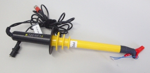
1.1 High Voltage probe

You need a HV probe to transform the high voltage output of the HVPS into a low voltage signal that can be fed to an acquisition device. The characterisation routines integrated in the GUI give the possibility to characterize the switching speed or the voltage regulation speed and stability. If you want to perform these measurements, you need to be able to measure dynamic signals. Therefore, you need a HV probe that is capable of measuring AC signals. We use a 10kV 1:1000 50MHz PR-55 probe from B&K Precision, but there are many other possibilities.

HV probes designed to be used with multimeters are suitable to perform the voltage calibration, but will not work for the other tests, because they require to measure voltage steps (i.e. the probe must have a large bandwidth).

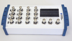
1.2 NI-DAQ system

You need a NI-DAQ system to acquire the analogue voltage on a computer. We use a NI USB-6212 BNC, but any system will do, as long as they have at least one analogue input. The entry-level NI USB-6000 should work fine. You must be sure not to exceed the voltage rating of your DAQ system when you connect the probe to it. However, NI-DAQ systems usually accept input signals in the +/- 10 V range, and HV probe commonly have a 1:1000 attenuation. Given that the HVPS with the highest rating (5kV) will output 5000 V or less, the voltage at the DAQ input will be between 0 V and 5 V, i.e. well within specification.

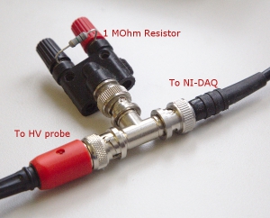
1.3 Impedance matching circuit

The dynamic HV probes, such as the 50MHz PR-55 we use are designed to be connected to an oscilloscope with a 1 MOhm input impedance (and if you are using a multimeter probe, it is likely designed to be connected to a multimeter with a 10 MOhm input impedance). NI-DAQ systems have a an input impedance >10 GOhm. Connecting a HV probe directly to a NI-DAQ system will lead to erroneous readings. In addition, it is recommended that signals connected to a NI-DAQ system have a low source impedance, which is not the case with HV probes.

You need to use an impedance matching circuit as interface between the probe and the NI-DAQ. In its simplest form, the impedance matching circuit is just a 1 MOhm resistor placed in parallel with the probe.

2 High Voltage Probe calibration

2.1 Performing the probe calibration

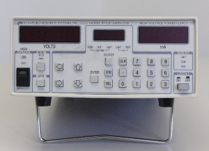
High voltage probes have a defined attenuation ratio (most of the time 1:1000), so a calibration is not absolutely necessary. However, much better accuracy can be obtained by performing a probe calibration. To perform a probe calibration, you will need a precision HV power supply, i.e. a power supply with an output voltage that you trust as being accurate. We use a Stanford Research Systems PS350/5000V power supply for this purpose.

• Connect your HV probe to the precision HV power supply, and to the impedance matching circuit. Connect the impedance matching circuit to the NI-DAQ.
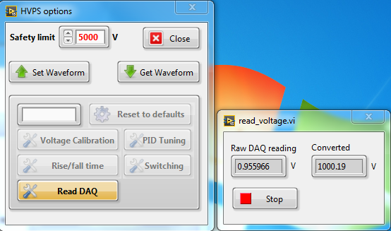
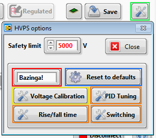
• For a set of voltages between 0 V and 5000 V (e.g. with steps of 100 V), set the HV power supply to the desired voltage value, and write down the low voltage value indicated by the NI-DAQ. NI provides tools to directly read a channel from a NI-DAQ connected to a computer so that you can read the analogue voltage. Alternatively, the HVPS interface provides the possibility to read the value of the high voltage probe from the configuration options (see screenshot). For this to work, there are two prerequisites: 1) The name of the NI-DAQ and the channel to read must be configured (see § 2.2 below), and a HVPS must be connected to the computer, or the interface main window won’t show up. The password to unlock the functions requiring the NI-DAQ is Bazinga!
  
• Plot the HV voltage value from the HV power supply (y axis) as a function of the low voltage value displayed by the NI-DAQ (x axis).
• Use curve fitting to find correction coefficients (see examples below)

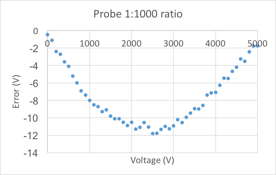
The graph below shows the error between the voltage calculated from the probe reading using the 1:1000 factor of the probe (i.e. without custom calibration). The approximation is acceptable, but there is an appreciable error, and a non-negligible average offset.

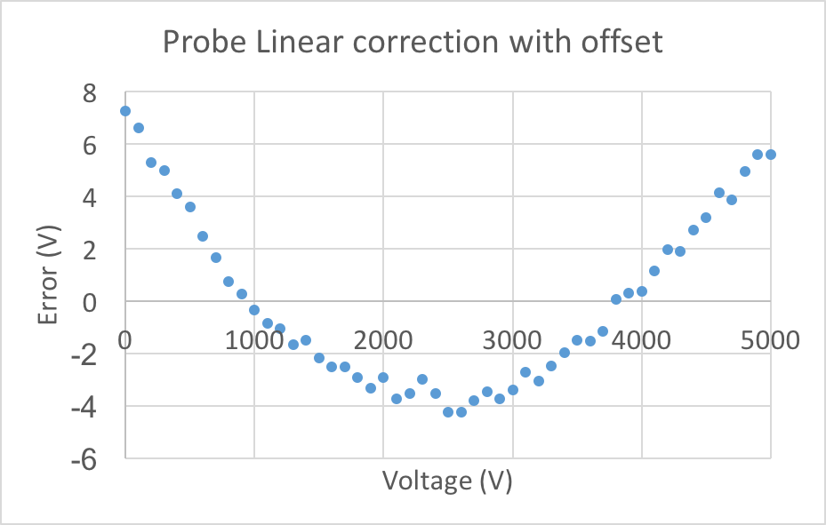
Based on the above information, a linear fit with offset, of the form y=c1 x + c0 is fitted to the data to account for the offset and a non-perfect ratio of the probe (see graph below). The error is much smaller. However, the error is not random, but takes the shape of a parabola, due to a non-linear effect of unknown origin.

Consequently, we fit the curve with a generic 2nd order polynomial of the form y=c2 x^2 + c1 x + c0. The error for this fit is given below. The error is considerably smaller than for the linear correction and comprised within a 3 V band.

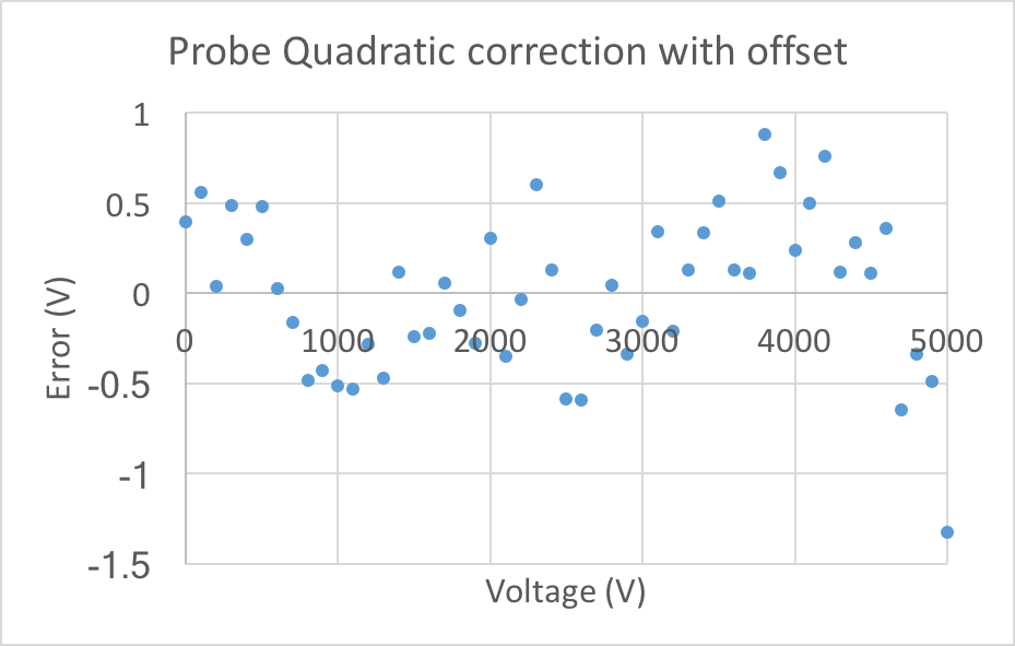
Given the previous observations, a generic 2nd order polynomial is recommended to calibrate your HV probe/impedance matching circuit/DAQ setup. The GUI interface integrates the possibility to have 2nd order polynomial to calibrate your probe. But by setting the right coefficient to 0, you can have a simple proportional calibration if you prefer. See the following section for how to enter your calibration coefficients so that your probe can be used for the automatic calibration.

2.2 Configuring the GUI to use the probe calibration

To keep the HVPS interface program as compact as possible, we have only included the components that are essential to run the program from a user point of view. This means that the LabVIEW components required to read data from a NI-DAQ system are not included, and the automatic calibration routines won’t work on a computer on which you install the interface, unless you also install NI-DAQmx, which is the package required to control NI-DAQ systems. You should have received a copy of NI-DAQmx with your hardware. Else, it can be downloaded from the NI website. You will also need the report generation toolkit to generate the excel file summarizing the results.

In the directory in which you have installed the HVPS interface, there is a folder named support. Open the file config.ini located in this folder. The first lines should look like the screenshot below:

The file allows you to enter calibration values for different probes (in case you have more than on HV probe, each with their own calibration. The probe name currently used by the programme is defined at the second line with:

• probe=”xxx”

where xxx represents the name you want to give to your probe, in this example it is PR55. You must then have a section in the file defining the parameters c0, c1, and c2 for your probe xxx defined by using the name of your probe in brackets, and then the 3 coefficients, each on one line:

• [XXX]
• c0=aa.aaaa
• c1=bb.bbbb
• c2=cc.cccc

The values of the coefficient c0 to c2 represents a quadratic fit obtained on your data from §2.1:
y = c0 + c1 x + c2 x^2
If you don’t want to calibrate your probe and want to use the ratio (e.g. 1:1000) provided by the manufacturer you can enter c0=0, c1=1000, and c2=0. If you only want a linear correction with offset, keep c2=0, etc.

In the [NI-DAQ] section you must enter the name of your NI-DAQ system (you can find that out with NI-MAX for example), and the analogue input channel to which the signal is connected. Our NI USB-6212 is called Dexter (but it hasn’t killed anybody… yet), and the signal is connected to the analogue input channel 0, so we have:

• [NI-DAQ]
• name=”Dexter”
• HVchan=”ai0″

Important: The program is reading a differential voltage from the probe. On the NI USB-6212, this is totally transparent, because it is equipped with BNC connectors. However, if you are using another unit that has screw terminals, you must connect the return signal to the input which is paired with the main signal. Refer to the manual of your NI-DAQ, but most likely, you have to add 8 to the main analogue input channel. For example, if you connect the main signal to ai0, you must connect the return signal (i.e. the ground of the impedance matching circuit) to ai8.

3 Performing the automatic calibration / characterisation

After having followed the instructions of section 2 above, it is time to calibrate and characterize your HVPS:

 

• High Voltage enable switch (s2): off position
• Connect the SHVPS to the computer (USB + 6VDC) and launch the HVPS interface
• Connect the HV cables to the output of the HVPS.
• Take your probe and connect the low voltage side to the input of your impedance matching circuit
• Connect the end of the HV cables to the probe: black to the ground of the probe and red to the HV terminal. Ensure that the HV (red) contact is well insulated, doesn’t touch any equipment and can not be touched by someone.
• Connect the output of the impedance matching circuit to the NI-DAQ, and the NI-DAQ to your computer.
• Power on the impedance matching circuit
• High Voltage enable switch: on position
• Open the HVPS options dialog box (green square), and if necessary, enter the password (Bazinga!) in the password input field (red) (we give the password here. The intention is not to make this secure, but just to prevent the general user of the HVPS to inadvertently change its configuration)
  

You are now ready to perform the automatic calibration / characterisation

• Voltage Calibration
• Setting of the PID regulator coefficient
• Characterisation of the rise and fall time of the voltage regulation (not the switching!)
• Characterisation of the rise and fall time of the high speed switching

4 Measurement file

The results of each of the tests mentioned above are saved in an excel file located in the support folder of the application (usually C:\HVPS_interface\support). Here are a few important points regarding the measurement file:

• The measurement file is named yymmdd_board_name_data.xls, with yymmdd the date at which the file was initially created.
• At the end of each measurement, the data is saved in the measurement file.
  • If no excel file with the name of the board being tested exists in the support folder, a new file will be created and the acquired data added to the file.
  • If a measurement file with the name of the board (irrespective of the date yymmdd) is present in the support directory, the new data will be added to this already existing file.
  • In this case, and if the measurement being done has already been done previously, the older measurement will be overwritten by the newly acquired data.
• The first tab (sheet) in the excel document summarizes the test which are included in the file, so that the user can see at once what are the file contents.
• The correct way to perform measurements is the following:
  • Perform all the tests that you need to characterize a board (typically, and especially if this is a newly assembled board, all of them)
  • Move the excel file from the support directory to a location where you archive all the measurements for future reference. It is important at this stage to move (and not copy) the file, so that the support directory doesn’t contain a file with the name of the HVPS anymore.
  • If at a later stage, the same HVPS is again characterized, then a new file will be created (instead of overwriting previous data, which would happen in case the first file remains in the support folder)
• The files are generated based on an Excel template (template.xltx). The template must not be open in excel when measurements are made, or the report generation will fail. And logically, the template must not be deleted from the support directory.